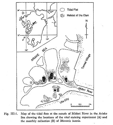
IV-1. Annual Patterns of Daily Growth Increments

In the previous chapter, the daily formation of growth lines was confirmed by a vital staining experiment. The next step in seasonal dating by means of the growth pattern of clams is to establish a standard zero date for a year. To do this, it is necessary to examine the seasonal variations of shell growth using a year-long pattern of daily growth increments (Koike, 1975b).

The clams used for investigation of the annual growth pattern were collected from a fixed site in the natural habitat of the species, on a tidal flat situated 0.5 km south of the clam-culture field where the staining experiment was carried out (see Fig. III-1). Specimens for analysis were collected once a month, during the ebb of the spring tide, from June, 1971, to May, 1972. The growth lines were observed as before by using the replica technique. The daily growth increments from the shell margin to the date of the preceding collection were measured with 5 specimens of the 4th-year shells selected from monthly specimens. Thus 12 sets of 5 specimens each, collected at one-month intervals, were examined to establish a year-long pattern of shell growth, and the mean thicknesses for each date were plotted in sequence.

The daily environmental records for sea-water temperature, salinity, rainfall and other weather records, and the tidal table were obtained through the courtesy of the Kumamoto Prefectural Fishery Station in Uto City.

The statistical analyses were processed by the HITAC-OS7 system at the Computer Centre, The University of Tokyo, using the CMREG1 (Multiple Regression 1), CPCREG (Regression on Principle Component) and CSPCTR (Cross Spectral Analysis) programs which were included in the HSAP (Hitachi Statistical Analysis Program) package.

The month-long patterns of daily growth increments for the 12 sets of 5 specimens were as shown in Fig. IV-1. The patterns for the 5 specimens of each monthly group were so similar that it seemed reasonable to use the mean values of daily shell growth. The annual pattern (Fig. IV-2) shows periodic sharp peaks from May to November and relatively weak peaks in the winter. The thinnest increments between the peaks were about 50 µm, and were relatively constant throughout the summer. The thickness of the daily growth increment tended to increase from May to July, and became thickest from July to August when it attained a maximum of 160 µm. The thickness decreased from October to November. During December and January, the thicknesses of the daily increments gradually decreased from 50 µm to 15 µm, and further decreased to 5-12 m from February to early March. From March to April, the thicknesses of daily growth increments gradually increased again from 15 µm to 30 µm, and the first peak in the new year appeared in early May, reaching 70 µm.

Seasonal variations of the sea-water temperature ranged from a maximum of 28°C to a minimum of 10°C during this year. During the summer season (from July to September), the temperature varied, ranging from 23°C to 28°C. The temperature gradually declined from October to December, and dropped to 12°C at the end of December. During the winter season (from January to March), it was 11-12°C. The minimum temperature (10°C) was recorded in early March, but it gradually rose again to as high as 20°C at the end of May. The seasonal shell growth trend indicated that the sea-water temperature was one of the basic influences on the thickness of the daily growth increments. Moreover, the growth minimum closely corresponded with the temperature minimum.

Tidal ranges in the Ariake Sea are +5.2 m to -0.25 m above and below the tidal datum level during the spring tides, and +3.8 m to +2.0 m during the neap tides. The sampling location depth was about +1.5 m; thus the collection area is always under water during the neap tides, while it should be exposed twice a day at the ebb tides during the spring tides. The cycles between the sharp growth peaks that appeared from May to November were about 12 to 18 days, suggesting tidal influence. Furthermore, shell growth minima corresponded with the spring tides in two-thirds of the cases.

Salinity at the fishery station near the collection area was usually constant, ranging between 24‰ and 26‰, except for the rainy season from June to August when it dropped to a low of 15‰. The influence of the salinity on shell growth, however, was not detectable even during the rainy season.

IV-2. Multivariate Analysis of the Relationship between the Annual Growth Pattern and Environmental Factors

The influence of 6 environmental factors on shell growth was examined in detail through multivariate analysis. Observation data (Table IV-1) on the thickness of daily growth increments, sea-water temperature, salinity and the height of tide were complete for an entire year, though some of the data on rainfall, cloud cover and wind were missing in the one-year series. Therefore, multivariate analysis was conducted for observation data sets for 363 days using shell growth, temperature, salinity and tide (Table IV-2A), and for sets from only 282 days using shell growth and the 6 environmental factors (Table IV-2B).

The correlation matrix for the 6 environmental factors (Table IV-2A) shows moderate correlations between temperature and salinity (-0.59), and between temperature and tide (+0.41), and weak correlations between salinity and rainfall (-0.28), rainfall and cloud cover (+0.28), and salinity and tide (-0.21). The apparent correlation of salinity and tide with the temperature could be caused by seasonal trends: salinity is low in summer and the tidal range is diminished during winter. The correlation of cloud cover and salinity with rainfall is thought to be a direct relationship.

Shell growth has the highest positive correlation with sea-water temperature (+0.80), and the lowest negative correlation with salinity (-0.53). It also has weak correlations with tide (+0.29) and rain (+0.22), although the latter two figures might possibly be related to the correlations among the environmental factors themselves.

Multiple regression analysis was carried out to examine the degree of influence of each environmental factor on shell growth, where shell growth was the dependent variable and the 6 environmental factors were the independent variables (Table IV-3). The selections in 5 cases (Selection 1 to 5) where environmental factors were selected arbitrarily produced similar multiple correlation coefficients. Moreover, the multiple correlation coefficient for Selection 5, where the dependent values were restricted to temperature and salinity, is the highest of the five. This indicates that temperature and salinity are the main influences on shell growth, and the other environmental factors are insignificant.

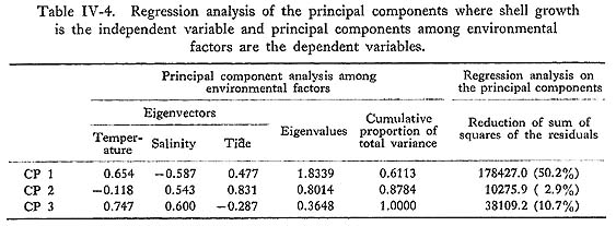
Regression analysis on the principal components was carried out to eliminate correlations among the environmental factors themselves from the correlations with shell growth. The results of the analysis where the dependent variable was shell growth and the independent variables were temperature, salinity and tide (Table IV-4) show that Component 1 among the environmental factors is thought to be a seasonal trend which has positive values for temperature and tide, and a negative value for salinity. Component 2 shows a high positive value for the tide. Component 3 shows positive values for both temperature and salinity, suggesting that weather factors are related. The cumulative proportion of total variance is 0.61 and 0.88 for Components 1 and 1 plus 2, respectively.

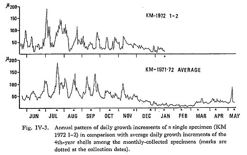
Table IV-4 gives the coefficients of regression equations using orthogonal components to standardized independent variables and the reduction in the sum of the squares of the residuals. It shows that Component 1 has a relatively strong effect on shell growth. Reduction due to component 2 is less than that of Component 3. Therefore, principal component analysis can be used to eliminate the correlations among environmental factors.

IV-3. Time Series Analysis for the Relationship between the Tidal Cycle and the Cyclic Growth Pattern

Multivariate analysis showed that temperature and salinity exerted the main influences on shell growth, and that, on the other hand, cloud and wind conditions had relatively insignificant effects. The effects of the tide did not appear in the multivariate analysis as clearly as seen on the annual pattern of daily growth increments, which showed cyclic peaks suggesting tidal effects. Thus, time series analysis was made for examining the relationship between shell growth and the tide.

Before the time series analysis was carried out, a daily growth pattern for the year for a single specimen (KM 1972 1-2) was established (Fig. IV-3). This was necessary because the average annual pattern was established by joining 12 successive one-month patterns. Although the cyclic pattern of the single specimen was not regular when compared with the averaged pattern, basic similarities were detectable. For example, sharp drops took place in both curves in mid July and in early August, and peaks in early July, in late to early August, and in late August were also noted.

To eliminate the influence of other environmental factors, especially sea-water temperature and salinity, a regression formula based on the results of the multivariate regression analysis was used. The observated value, that is, the thickness of the daily growth increment, was compared with the estimated value calculated using the multivariate regression formula with the correlation coefficient of the independent variables, temperature and salinity. The differences between the estimated values and observed values were then introduced as the values at which the influence of the independent variables was eliminated.

The results of this procedure (Fig. IV-4) showed that the height of the cyclic peaks of the residual series became uniform around the mean of the observated series, compared with the pattern of the observated series which had a seasonal trend. This indicated that multivariate regression analysis can be useful in preparing a series when specific environmental factors have to be eliminated.

The first of the time series analyses is the correlogram (Fig. IV-5). This is used to indicate the periods of cycles and the degree of repetition in the periodical patterns. The correlogram of the tidal series shows positive peaks of high correlation on the 14th and 28th lag day, with the latter peak being slightly higher than the former. On the other hand, the correlogram of the daily growth increment series shows relatively weak peaks, compared to those of the tidal series. There was a clear peak on the 28th lag day, but the peak on the 14th lag day was barely detectable. These peaks retained negative values around the 42-43rd lag day, contrary to the tidal pattern.

When the observation series of daily growth increments is compared with the revised series, a similar correlogram pattern, with only slight variations, is seen.

The second step in the time series analysis was power spectrum analysis (Fig. IV-6), which gives the intensity of the period of a cycle by scanning the frequency (observated cases / i lag). The intensity of peaks produced by the power spector analysis was affected considerably by the procedure in preparing the data for the time series analysis. In the present survey, a 156-day series of growth increments from May to October, instead of the full one-year pattern series, showed sharp peaks in a power spectrum. The power spectral pattern of the tidal series has sharp peaks at 28-, 14- and 7-day frequencies. Among these three, the power spectral peak at the 14.0-day frequency is highest. The power spectrum pattern of the average daily growth increment series has weaker peaks at 28-, 14- and 7-day frequencies than the tidal series, both in the observation data series and in the revised series. When the original observation series was compared with the revised series, the latter showed slightly clearer peaks in the power spectral pattern.

On the other hand, the power spectrum estimates of the daily growth increment series of KM 1972 1-2 indicate relatively apparent peaks at the 28- and 14-day frequencies. Moreover, the power spectral pattern of the revised series has more con spicuous peaks than those of the observation series and also has peaks at the 28- and 14-day frequencies.

In the third step, cross-spectrum analysis (Fig. IV-7) was used to examine the cyclic response between the tide and shell growth. The co-spectrum of the tidal series and average shell growth series has a sharp negative peak for the 28.0- and 14.0-day frequencies. These results are also well represented in the amplitude of the cross-spectrum.

In the cross-spectrum analysis, the intensity of the peaks of the 14-day frequency, both in the co-spectrum and the amplitude of cross-spectrum, was higher than those on the 28-day frequency. This was contrary to the results of the power spectrum analysis.

IV-4. Recognition of the Annual Growth Minimum

In order to set a standard zero point for seasonal dating, a year-long pattern of daily growth increments with specimens of which collection dates were known was made and compared with environmental records in this chapter. To examine the annual pattern of daily growth increments, it is preferable to satisfy the following conditions. First, the periodicity of the growth increments must not change its rhythmic manner. Primary growth lines in M. lusoria are conspicuous in the inner zone and easily distinguished from the tidal lines, and these primary lines are confirmed as showing a daily periodicity. Second, the shell must show continuous growth throughout the year, without stunting due to weather condition, especially in winter. The annual pattern of growth increments of M. lusoria shows a maximum growth of 250 µm, and continuous growth of 5 to 15 µm even in the winter, at least in the 4th year shells. Winter growth indicates a gradual decrease toward the mid-winter. This minimum growth corresponds to the minimum sea-water temperature, as multivariate analysis indicated that sea-water temperature is the main environmental parameter. Therefore, a standard zero date for seasonal dating should be set at the point of minimum growth in the annual pattern.

The influence of high temperature during summer was noted in the present samples of M. lusoria. This is another indication that further investigation of annual growth increment patterns will give detailed information on environments: Kennish and Olsson (1974) used the growth increments of Mercenaria mercenaria as a monitor on environmental conditions, showing that the summer growth rates of M. mercenaria from area subjected to thermal effluents were lower than those from unaffected areas.

House and Farrow (1968) felt that tides exerted their greatest influence in shell growth through annual patterns of daily growth increments. The influence of the tide is also reported, especially in young shells, during the period of rapid growth from spring to autumn (Whyte, 1975;Evans, 1972 and 1975; Farrow, 1972). Although the effects of the tide on shell growth in the present species did not appear in the multivariate analysis, a cross-spectrum analysis between the tide and shell growth showed that the cospectrum had sharp negative peaks for the 14- and 28-day frequencies. Estimated values calculated by multiple regression analysis where sea-water temperature and salinity are independent variables is useful to eliminate the seasonal trend or influence of sea-water temperature and salinity to obtain precise information on the tide with the amplitude given by the time series analysis. Dolman (1975) who established a flow diagram of growth increment analysis using time series analysis, estimated the tidal conditions by the phase and amplitude of fortnight periodicity in the shell growth of Cardium edule.